

In today’s industrial landscape, efficient and reliable automation is essential for optimizing processes and maximizing productivity. Programmable Logic Controllers (PLCs) play a crucial role in achieving these goals. PLC programming, often done using ladder logic, is the process of creating instructions and logic that enable PLCs to perform specific tasks. In this article, we will explore the fundamentals of PLC programming, the tools and software involved, and the benefits it brings to industrial facilities. Whether you’re new to PLC programming or looking to enhance your existing skills, this article will answer the question of how one can learn PLC programming & provide valuable insights and guidance.
We will begin with the basics of logic circuits, described in the literature as “Logic Gates”.
Logic Gates
Logic gates are an essential component in the field of programmable logic controllers (PLCs) programming. PLC programming involves creating ladder logic programs to control and automate various industrial processes. In this article, we will explore the fundamentals of logic gates and how they tie into PLC programming, while also teaching the basics of PLC programming.
Logic gates are electronic circuits that perform basic logical functions. They are the building blocks of digital electronics and play a crucial role in controlling the internal logic of a PLC. There are several types of logic gates, including AND, OR, NOT, XOR, NAND, and NOR gates. Each gate operates based on specific logical rules and produces an output based on the inputs it receives.
In PLC programming, logic gates are represented graphically using ladder logic diagrams. Ladder logic is a programming language that mimics the electrical circuits with which PLCs were originally designed to replace. It uses symbols to represent the different components and instructions in a program.
Let’s take a closer look at some of the commonly used logic gates and how they are represented in ladder logic:
1. AND Gate:
The AND gate produces an output only when all of its inputs are TRUE. In ladder logic, the AND gate is represented by a series connection of two or more normally open (NO) contacts. For example, if contact A and contact B are both normally closed, the output of the AND gate will be true only when both contacts are closed. The output is connected to a coil or another instruction.

2. OR Gate:
The OR gate produces an output if any of its inputs are TRUE. In ladder logic, the OR gate is represented by a parallel connection of two or more normally open (NO) contacts, meaning that any of the contacts being closed will result in a true output. For example, if contact A and contact B are both normally open, the output of the OR gate will be true when either contact is closed. The output is connected to a coil or another instruction.

3. NOT Gate:
The NOT gate, also known as an inverter, produces an output that is the opposite of its input. In ladder logic, the NOT gate is represented by a normally closed (NC) contact. When the input contact is closed, the output will be open, and vice versa. The output is connected to a coil or another instruction.

4. XOR Gate:
The XOR gate produces an output that is TRUE if only one of its inputs is TRUE. In ladder logic, the XOR gate is represented by a combination of normally open (NO) and normally closed (NC) contacts. For example, if contact A and contact B are both normally open, the output of the XOR gate will be true when either contact A or contact B is closed, but not both. The output is connected to a coil or another instruction.

5. NAND Gate:
The NAND gate produces an output that is FALSE only when all of its inputs are TRUE. In ladder logic, the NAND gate is represented by a series connection of two or more normally closed (NC) contacts. For example, if contact A and contact B are normally closed, the output of the NAND gate will be false only when both contacts are closed. The output is connected to a coil or another instruction.

6. NOR Gate:
The NOR gate produces an output that is TRUE only when all of its inputs are FALSE. In ladder logic, the NOR gate is represented by a parallel connection of two or more normally closed (NC) contacts. For example, if contact A and contact B are normally open, the output of the NOR gate will be false only when either contact A or contact B is closed. The output is connected to a coil or another instruction.

Now that we understand the basics of logic gates and how they are represented in ladder logic, let’s move on to the basics of PLC programming.
PLC programming involves designing and creating ladder logic programs that control and automate industrial processes.
Normally Open & Closed Contacts
Normally open and normally closed contacts are fundamental components of Ladder Logic PLC programming. They are used to represent the status of input or output devices in a control system. These contacts are typically used in ladder logic programming, one of the commonly used programming languages in PLCs.
A normally open contact, also known as an NO contact (or an “Examine if Closed” bit), is represented by a symbol that looks like a switch with an open gap. This symbol indicates that the contact is open when the associated input or output device is not activated. In ladder logic programming, an NO contact is used to represent a condition that must be true for a specific operation to be executed.
Each bit in a PLC program is assigned an address, in this case the first bit used in our ladder logic would have an address of I0:0.
Essentially, this means “Input Bit #1”.
Indeed, both inputs and outputs are considered memory bits within the PLC. In the provided illustration, the “examine if closed” instruction is associated with the memory address I0.0 as its condition. This particular address is reserved for the PLC’s primary input.
The procedure is as follows:
- Upon initiating the PLC scan cycle, the PLC examines the status of all its inputs.
- Subsequently, it records the corresponding boolean values (either 0 or 1) of these states in its memory.
- If an input registers as LOW, its corresponding memory bit will register as 0. Conversely, if the input is HIGH, its memory bit will be recorded as 1.

On the other hand, a normally closed contact, also known as an NC contact (or “examine if open” bit), is represented by a symbol that looks like a switch with a closed gap. This symbol indicates that the contact is closed when the associated input or output device is not activated. In ladder logic programming, an NC contact is used to represent a condition that must be false for a specific operation to be executed.

These symbols are used in ladder logic diagrams to create logical relationships and control the flow of operations in a PLC program. By properly configuring normally open and normally closed contacts, programmers can define the conditions under which certain tasks or operations should be executed in an automated control system.
Coils & Output Bits
In addition to the NO & NC contacts mentioned previously, another type of symbol is used in ladder logic to represent activation of the PLC output.
As you will see in the ladder logic example to follow, once our contacts are made “true” and electricity is allowed to flow across the ladder from left to right, a final instruction is required in order to make the PLC send its output signal to the real world, activating the desired results from field equipment.
In other words, once this coil symbol is made true in the program, real world actions may occur.

As shown below, the coil symbol is positioned on the rung’s right-hand side. This implies that any preceding instructions on the same rung serve as conditions for that specific instruction.
Taking our example into account, the outcome of the “examine if closed” instruction would be the resultant condition. Once the PLC has stored the statuses of all inputs, the program commences its operations. The initial instruction to be processed is the “examine if closed” or what’s also known as “normally open.” The outcome of this directive mirrors the status of the saved memory bit.
The term “normally open” is fitting for this instruction. In its standard state (with a memory bit of 0), the contact remains open, resulting in an output of 0. However, if the memory bit is 1, the contact engages, producing an outcome of 1.

Getting Started
To program a PLC, you will need a programming device. This can be a dedicated device provided by the manufacturer of the PLC, or it can be a personal computer with PLC programming software installed.
The software allows you to write, test, and debug PLC programs before transferring them to the actual PLC hardware. Typically, a programmer or maintenance electrician will have a dedicated programming terminal or laptop with the appropriate software installed for their system. A program can be written or modified & tested in this environment after which it is transferred by USB to the active PLC.
PLC programming software allows users to write, test, and debug programs in a graphical form. It provides a user-friendly interface that simplifies the programming process and allows for efficient troubleshooting. With the software, users can easily create, modify, and monitor the internal logic of the PLC.
Once you have your programming device and software, you can start creating your PLC program. This involves writing instructions that define the internal logic of the PLC. These instructions can range from simple on/off commands to complex mathematical calculations.
It’s important to note that PLC programming languages vary depending on the manufacturer and model of the PLC. However, the most common languages include ladder logic, function block programming, and structured text. It’s important to choose the right programming language for the task at hand.
Ladder logic is often used for simple on/off control and basic logic operations. Function block programming is ideal for tasks that involve mathematical calculations or data manipulation. Structured text is best suited for complex applications that require advanced programming techniques.
Ladder Logic
Ladder logic is the most widely used language in PLC programming. It is a graphical language that represents the logic of a program using ladder diagrams. Ladder diagrams consist of rungs, which are horizontal lines that contain instructions. These instructions are represented by symbols, such as contacts and coils.
In ladder logic, instructions are represented by symbols called contacts and coils. Contacts are inputs to the ladder logic program and can be either normally open (NO) or normally closed (NC). Coils, on the other hand, are outputs of the program and represent devices or actions that the program controls.
Placing contacts and coils in ladder logic programming allows for the creation of complex control systems. By using different combinations of logic gates, complex behaviors and conditions can be achieved. This makes ladder logic a powerful and flexible programming language for programmable logic controllers.
Ladder logic programming is widely used in industrial facilities for controlling and automating various processes and equipment. It offers a visual representation of the control system, making it easier to understand and modify.
One of the key advantages of ladder logic programming is its ability to represent the internal logic of a control system in a simple and intuitive manner. The graphical form of ladder logic allows users to easily identify and troubleshoot issues within the program.
Another advantage of ladder logic programming is its compatibility with various programming devices. PLCs can be programmed using a personal computer or a dedicated programming device. This flexibility allows for easy integration of ladder logic into existing control systems.
Ladder logic also offers a wide range of instructions and tools that can be used to program the PLC. These include timers, counters, arithmetic operations, and comparison instructions. These instructions enable the creation of complex control systems with precise control and monitoring capabilities.
Furthermore, ladder logic programming languages are standardized and widely supported by different manufacturers. This means that programs created using ladder logic can be easily transferred between different PLC models and brands. This makes it easier for industrial facilities to maintain and upgrade their control systems without the need for extensive reprogramming.
In addition to ladder logic programming, there are other programming languages that can be used in programmable logic controllers (PLCs). Some examples include structured text (ST), function block diagram (FBD), and sequential function chart (SFC). Each programming language has its own advantages and may be more suitable for certain applications.
Understanding Ladder Logic Diagrams
One notable distinction between ladder logic diagrams and traditional electrical schematics is their orientation. While electrical schematics are commonly presented in a horizontal format, ladder logic diagrams are vertically structured. The reasons for this vertical arrangement include:
Improved Readability
Reading ladder logic vertically aligns with the natural motion of the eyes, which move from left to right before proceeding to the next line. This is particularly relevant for individuals from regions where the reading direction is left-to-right.
Digital Representation
When designing ladder logic using computer software, you typically create one line or rung at a time. As more rungs are added, they stack atop one another, resembling a ladder. To view extensive ladder diagrams, scrolling vertically provides a more intuitive experience.
Sequence of Operations
Positioning ladder logic vertically establishes a clear execution order. The PLC processes the ladder logic by beginning at the top and working its way downwards. Specifically, this vertical setup dictates the sequence in which the PLC carries out the ladder logic commands.
Delving into Relay Ladder Logic
While vertically oriented ladder diagrams might remind many of electrical schematics, there are distinct differences. Instead of approaching ladder logic as merely vertical electrical schematics, it’s beneficial to grasp it from a unique perspective, which I’ll elaborate on in this guide.
Two main differences between electrical control systems and PLCs are:
- A PLC processes one ladder logic rung before moving to the subsequent rung.
- Contrarily, in electrical systems, several pathways (lines) can be activated concurrently.
With these essential distinctions, we’re set to dive deeper into ladder logic.
Getting Started with Ladder Logic
Upon initiating a ladder logic design, you’ll notice two parallel vertical lines. Your ladder logic will be positioned between these lines. As you sketch out your ladder logic, you’ll form vertical links connecting the two main lines, termed as rungs, analogous to the steps of a ladder. Each rung accommodates various ladder logic symbols to formulate the desired logic.
Observably, I’ve numbered each rung to denote the sequence in which the PLC device processes the ladder logic. You might have heard about the PLC’s scan cycle or scan duration. Essentially, the PLC first reviews its inputs, followed by executing the program to determine outputs. So, how does the PLC process our ladder logic?
It processes one rung sequentially.
This is a pivotal ladder logic principle: the PLC processes each rung individually, one after the other, and indeed, tackles one symbol at a given moment.

Function Block Diagram
In addition to ladder logic, another commonly used programming language in PLC programming is function block programming. Function block programming allows users to create complex logic by using pre-defined blocks or instructions. These blocks can be connected together to create a program.
Function block programming is often used in PLC programming to create reusable code and modularize the logic. It allows programmers to create custom blocks for specific tasks and easily incorporate them into different programs. Function block programming is especially useful for tasks that involve mathematical calculations or data manipulation. It allows for the creation of reusable and modular code, making it easier to maintain and troubleshoot PLC programs.
OR Block
The first function block I will introduce you to is the OR Block.
Remember the OR gate we discussed at the beginning of this article? An OR Block functions in the exact same way. If either of the input pins on this block become true (A Boolean value of 1), then the output also becomes true.

AND Block
Second is the AND block. In the same way that our AND logic gate required a Boolean value of 1 on each input pin to create a value of 1 on the output, this block needs each input to be true before the output becomes true.

NOT Block
There may be times when you want to reverse either the input or output of a block. In this case the NOT block may be used in order to achieve that.
Think back to the NOT gate mentioned at the beginning of this article, when the input becomes true the output of this block will become NOT true, (A Boolean value of 0). Likewise, when the input is NOT true, the output of this block will in fact become true.

XOR (Exclusive OR) Block
The XOR block is a variant of the OR block we’ve already discussed. While the OR block requires one OR the other input pins to be true in order to provide a true output the XOR works a little differently.
In the case of an XOR should both input pins be true, the output will always be false.

NAND Block
5th on the list is a NAND block. NAND meaning “Negated AND”.
This block works the exact same way as the AND does, but the output value will always be reversed. Should an AND block have a true output given the inputs, a NAND will have a false value in its place.

NOR Block
Using the same principle as the NAND block above, the NOR (Negated OR) block functions the same way as an OR block does but will have a reversed value on the output.
Should an OR block have a value of 1 on the output, a NOR will give a value of 0.
Bistable Function Blocks
Next up in our discussion are bistable blocks, which one could perceive as the most basic memory forms. Their output can be either set or reset, and the output (Q) retains the prior state of the set input (S1).
Activate S1, and Q1 becomes set. Even if S1 reverts to a false state afterward, the output remains true. In essence, Q1 holds the record of any activity on S1. This is the rationale behind considering bistables or flip-flops as memory elements.
Set/Reset
This block is denoted as SR, standing for set/reset. Here’s its visualization: For a clearer grasp, let’s dissect the function block. The SR block’s anatomy reveals its composition from two distinct logic blocks: an AND function and an OR function.

The AND function’s output feeds into the OR function. Notably, one of the AND function inputs is Q1, which also serves as the block’s overall output.
Many term this as a flip-flop function. Q1 retains the knowledge that S1 was once true, up until the reset (R) becomes true, prompting Q1 to reset. Recognizing that the output (Q1) has this retention capability, I often refer to this block as a rudimentary memory block. When both inputs are simultaneously true, what’s the outcome?

For SR-blocks, the set command takes precedence. So, with both inputs being true, the output gets set.
However, this may not always be the desired function, leading us to another variant.
Reset/Set Functionality
There are instances when you’d prefer the output to reset if both inputs (S1 and R) are active. Hence, the existence of the RS block.

Its operation closely mirrors that of the SR block, with the only difference being its priority leaning towards reset over set.

Edge Detection
In both electronics and PLC programming, detecting edges is invaluable. Here, we’re referring not to physical edges but to signal transitions.
Consider an input connected to a push button, and you aim to track its press frequency.
Typically, one might connect this input to a counter function block (more insights later). However, remembering the basic dynamics of a PLC — possessing a scan or cycle duration — is essential.
Though this duration is brief (around 20-50 ms), a push button press usually lasts longer (around 100-200 ms). As a result, several scan cycles capture this input as active.
Consequently, with each PLC cycle that hits the counter block, the counter increments due to the active input. A single button press could result in multiple counts.
To counteract this, edge detection blocks become crucial.
R_TRIG Function Block
A rising edge in a digital signal can be observed. Often termed the positive edge, it’s witnessed when signals transition from false (0) to true (1), like a voltage leap from 0 to 5V.

This edge is evident right at button press. On detecting a rising edge, the output sets but momentarily due to the swift edge transition. Subsequent scan cycles, despite an active input, don’t re-set the output. The output generates a pulse only upon detecting a rising edge.
The block essentially “recalls” any positive edge on the input. Thus, to trigger the output again, the input must shift from false to true. In our context, this means releasing and then pressing the button.

F_TRIG Function Block
Besides rising edges, falling edges are also detectable. The transition of signals from true (1) to false (0) indicates a falling or negative edge.

It too operates by sending a pulse to the output in response to a falling input edge. This block proves handy when a specific action is needed upon another’s cessation.
For instance, imagine wanting a yellow light to illuminate when a motor halts, but only post its activation. So, the yellow light should shine precisely when the motor stops.
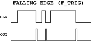
Solution: Implement an F_TRIG to spot a falling edge on the motor output, generating a pulse that activates the yellow light’s output.
Timer Function Modules
In our previous discussions, we emphasized ensuring a signal did not exceed the scan duration. However, there are instances where you might want to dictate the signal’s duration or its occurrence timing. Enter the realm of timer function modules. These timers are a staple in PLC programming and come in three distinct variations.
For a more in-depth exploration of timers, complete with PLC simulations, consider perusing the article dedicated to PLC timers. It provides video tutorials on the on-delay timer, off-delay timer, and pulse timer.
While some contend that mastering just one timer is sufficient since its foundational function can be adapted to emulate the others, I advocate for familiarity with all three since they’re all elaborated in IEC 61131-3 and are commonly available in most software platforms.
Pulse Timer (TP)
The inaugural timer we’ll discuss is the pulse timer, designed to produce a pulse of a specified duration.
This timer requires two inputs and furnishes two outputs. Up until now, we’ve only encountered function modules with boolean inputs and outputs. This holds true for the TP block’s IN and Q, but the PT and ET diverge slightly, accepting the TIME data type.
PT (Preset Time) is the block’s input, where you define the duration for the pulse at Q. When the input IN activates, the output Q engages for the PT duration. ET, representing Elapsed Time, denotes the active duration of Q.

For instance, if you desire a ventilation fan to run for 10 minutes, you’d input 10m in PT and link the fan to output Q. Often, monitoring the fan’s operational duration proves useful, which is where ET comes into play. The pulse timer’s operation can be further understood via its detailed time diagram.

On Delay Timer (TON)
The subsequent timer variant is the On Delay Timer, often abbreviated to TON. Contrary to setting the pulse’s duration, this timer introduces a delay prior to the pulse’s initiation.
Upon input activation, the timer commences its countdown. Once the PT duration concludes, the output Q activates—hence its naming rationale.

It powers the output following a specified delay. The on-delay timer retains the same input and output configuration as the pulse timer, inclusive of the ET to track elapsed duration.
The below diagram for the on-delay timer offers a clearer visualization of its operation. Some assert that this particular timer is all-encompassing, but before delving into that argument, let’s discuss the third timer variant.

Off Delay Timer (TOF)
The operational essence of the off-delay timer (TOF) mirrors the TON, with a singular, distinguishing feature.
It deactivates the output after a specific delay.

Upon input activation, the output immediately engages. If the input remains active, the output persists until the PT duration concludes. Subsequently, the output disengages. At a glance, the off-delay timer might seem a replica of the pulse timer (TP). They are indeed analogous, but an essential distinction exists.
While the pulse timer’s output remains engaged for the PT duration, even if the input becomes inactive mid-timing (as it detects input’s rising edge), the off-delay timer ceases its countdown if the input reactivates.

These three timers are canonically described in IEC 61131-3. In theory, using some ladder logic, all these functionalities can be replicated using just the on-delay timer.
Counter Blocks
Counting is a core element in PLC programming. Questions like “How many items have been produced by the machine?” or “At what stage is the tool currently?” underscore the significance of counters in PLC applications.
The IEC offers three standard counter modules: one for incrementing, one for decrementing, and one that can do both.
Let’s delve into the incrementing counter first.
Incrementing Counter (CTU)
This module comprises three input channels and two output channels. Despite appearing intricate, every channel is pivotal for the counting process. To grasp its functionality, let’s first understand the basics.
For every pulse detected on CU, CV increments by one unit. Once CV reaches or surpasses PV, Q activates.

The CU input is designed to identify a rising pulse. Upon its detection, the CV output escalates by one unit. To facilitate this, the CV output must adopt an integer data type.
Given that the integer is a 16-bit representation (with the inaugural bit marking signed/unsigned distinction), the maximum count attainable is 32,767. Both PV input and CV output embrace the integer data type. PV establishes the threshold at which the boolean output Q triggers. The reset channel (R) is deployed to revert CV to zero. Typically, counting initiates from zero, ensuring CV mirrors the pulse occurrences on CU.
For those inclined towards text-based coding, the structured text representation for this function block is as follows:
***
IF R THEN
CV := 0;
ELSIF CU AND (CV < PVmax) THEN
CV := CV + 1;
END_IF;
Q := (CV >= PV);
Decrementing Counter (CTD)
Counting isn’t solely about addition; there are scenarios requiring subtraction. For instance, you might desire a PLC application to execute an action for a specified number of times, making the decrementing counter invaluable.
Every pulse on CD reduces CV by one. When CV dwindles to zero or less, Q is activated.

This operates analogously to the incrementing counter but inversely, decrementing by one instead. This introduces a distinction: from what value should decrementing commence?
While incrementing typically starts from zero, decrementing requires a predefined value to decrement from. Hence, the LD input is present. When LD is activated, CV mirrors PV. The structured text representation for this block is:
***
IF LD THEN
CV := PV;
ELSIF CD AND (CV > PVmin) THEN
CV := CV – 1;
END_IF;
Q := (CV <= 0);
Now, having understood both incrementing and decrementing processes, let’s explore the combined counter module.
Bi-directional Counter (CTUD)
On occasions, the flexibility to count both ways – increment and decrement – is beneficial. Consequently, IEC introduced an official bi-directional counting module.

This module features 5 inputs and 3 outputs, maintaining naming consistency with its predecessors. It’s essentially a fusion of the two prior modules, with each input/output retaining identical functionalities. To truly comprehend its workings, let’s view its structured text representation:
***
IF R THEN
CV := 0;
ELSIF LD THEN
CV := PV;
ELSE
IF NOT (CU AND CD) THEN
IF CU AND (CV < PVmax) THEN
CV := CV + 1;
ELSIF CD AND (CV > PVmin) THEN
CV := CV – 1;
END_IF;
END_IF;
END_IF;
QU := (CV >= PV);
QD := (CV <= 0);
***
At a cursory glance, this might seem intricate. However, it merely amalgamates the functionalities of both incrementing and decrementing counters. CU increments CV by one, while CD reduces CV by the same. Both outputs, QU and QD, are determined by the same conditions as in the prior counter modules.
Comparison Blocks
I often perceive the upcoming function blocks as posing queries. Does A match B? Is CV larger than PV? Let’s dive into number comparison!
Indeed, comparison is a concept we’ve previously encountered in several blocks. Consider the OR block, which juxtaposed two boolean values. If their combined value was 1, the output got triggered.
But FBD isn’t limited to boolean data type comparisons. We can analyze all genuine numbers (apologies to math enthusiasts, no imaginary numbers for now) and a majority of other data types. Not only is this feature useful, but it’s also a tool you’ll find yourself using frequently.
A commonality among comparison blocks is that they all consist of two or more inputs and a singular output. These inputs can accommodate any basic data type, while the output remains boolean. One must tread cautiously when juxtaposing data types due to potential complexities.
Now, let’s kick things off with the primary comparison block:
Equality

The function block for equality helps determine if two variables have the same value. If they match, it triggers the output. A simple way to understand this block is by posing the question:
Does IN1 match IN2?
While it might seem straightforward, it’s essential to ensure the data types being compared are compatible. Frequently, integers are the primary data type used for these comparisons. For instance, to trigger an output when a machine reaches step 12, IN1 represents the current step, and IN2 is set to 12.
Notice the three dots between inputs? This signifies that the block can handle more than just two inputs. For the output to activate, all inputs must match. The structured text description of this function is:
OUT := IN1 = IN2 = … = INn
However, comparing different data types might introduce challenges. Comparing two real data types, for example, might seldom yield exact matches.
This is because real data types represent floating-point numbers. So, if you wish for an action to occur at 80 degrees, using real data types would mean it must hit precisely 80.0 degrees. For more flexibility, use compare blocks to compare within a range, rather than a single value.
Yet, for integers or words, the equality block proves handy.
The Inequality Block (<>)
But what if your goal is to ensure certain numbers don’t match? One could reverse the output of the equality block, but that’s not intuitive. Thankfully, there’s a block designed for this exact purpose.
This block’s functionality mirrors its predecessor but checks for differences rather than matches. To grasp its essence, ask:
Does IN1 differ from IN2?

If they don’t match, the output activates. Once they do, the output deactivates. In structured text, inequality is symbolized as <>, which resembles the “!=” notation in many programming languages. Note that this block only accepts two inputs.
The Less Than Block (<)
As mentioned, equating real data types can be tricky. The solution? This block allows you to determine if a variable falls within a numeric range.
Its official title is the increasing sequence, but “less than” is more intuitive. Essentially, it checks:
Is IN1 smaller than IN2?
This block excels with real numbers, for instance, to see if the temperature is below 80.5 degrees. When extended to more than two inputs, the name “increasing sequence” becomes more apt, as IN1 must be less than IN2, which in turn must be less than IN3, and so on.

This block is described in structured text as follows:
OUT := (IN1 < IN2) AND (IN2 < IN3) AND … (INn-1 < INn)
The Greater Than Block (>)
This block’s principle is the opposite of “less than”. It verifies:
Is IN1 larger than IN2?
Similar to its counterpart, this block can accommodate multiple inputs. The values should form a decreasing sequence for the output to be set. When combined, the “greater than” and “less than” blocks can validate if values lie within a specific range, like if a temperature is between 90 and 100 degrees.

In practice, comparison blocks are often paired. For instance, the equality block might team up with either the “less than” or “greater than” block. Despite being block combinations, they sometimes have individual function blocks such as:
Less than OR equal to
Greater than OR equal to.
This block is represented in structured text using the following code:
OUT := (IN1 > IN2) AND (IN2 > IN3) AND … (INn-1 > INn)
Selection Function Blocks
Comparing two or more values is useful. But sometimes, instead of comparing, you will have to choose between values. The selection function blocks give you that opportunity. What they all have in common is that they give you the option of selecting a value.
With or without conditions. The essence of these blocks is really just an assignment. You will select one of the inputs and assign it to the output of these blocks.
Move
The first and most simple selection block is the move function block. In fact, you have already seen this block before. Or at least a block with the same functionality.
The assignment function block. What this block does is that it assigns the input value to its output. And guess what. This block does exactly the same thing. You might wonder why FBD provides two blocks with the same function. They are also similar, but with one crucial difference.
While this block can be used with any data types, the assignment block can only be used with boolean data types. With the move block you can move any data type to any data type.
For you that like structured text, the representation of the block looks as simple as this:
OUT := IN

As you can see this block only has one input and one output. The concept of selection doesn’t really apply to this block, since you only have one value to select. Many times though you will be able to add more outputs to the move block.
A moving block can thereby be used to move a value to different places. When I said this block works with any data type, I really meant it. You can move values from any data type to any data type.
You don’t even have to put the same data type in the output as the input. You’re free to move e.g. an integer to a real, a TIME to a double word and so on. This makes the moving block a bit tricky.
You have to be really careful when moving from one data type to another. For beginners, I highly recommend that you only move values to the same data type as the input. As a matter of fact, I would rarely recommend mixing data types even for professionals. It just makes your PLC program complicated.
Binary Selection (SEL)
Binary selection drags us a little closer to the concept of selection.
It gives you the opportunity to select between two values to then assign to an output. The name indicates that you with a binary (boolean) input can select one of two input values. Therefore this block has three inputs. One condition (G) and two values (IN0, IN1).

The condition takes a boolean data type and is used to select between the two values. You will most likely have noticed that the input names are a bit different than with the other function blocks.
That is only to make the block easier to understand. Since the condition (G) can take two different values 0 and 1, it makes sense to call the inputs IN0 and IN1. If G is 0 the input IN0 will be selected. And if G is 1 the input IN1 will be selected. The value of the selected input will then be assigned to the output (OUT).
Again, this functionality can be represented in structured text:
IF G = 0 THEN OUT := IN0 ELSIF G = 1 THEN OUT := IN1 END_IF;
Extensible Multiplexer
In some cases, you may even have more than two values you want to select from.
This is where the extensible multiplexer comes into the picture. You might even find the word multiplexer familiar if you know a few digital electronics. And this block has the same functionality – to choose one out of many inputs.

Like the previous block, this block has two types of inputs. A condition (selector) and some input values. The block selects one of N inputs depending on the value of the selector.
Unlike the binary selector the condition input, named K in this block, can not only take a boolean data type. In fact, it can take up any elementary data type. Although the only data type that really makes sense to use here is an integer. As you have to choose between inputs from IN0 to INn it only makes sense to give the condition K a whole number.
Actually it is only valid to give K a number between 0 and n.
The concept of the function may look like this:
OUT := INK
Where K has to be within the range 0 – n, where n is the number of inputs.
Extensible Minimum Function (MIN)
So far you have seen how to select values using a condition input. That input could be either binary or an integer depending on how many inputs you have to choose between.
But sometimes you will want to select a value depending on the values themself. It could be that you want to select the highest or the lowest value among different variables.
With the next two function blocks, you can do exactly that.

Choosing the variable with the smallest value is something that I can guarantee, that you will use at some point. The official name for this function block is extensible minimum, but often just called minimum or MIN.
It is called extensible because you can add any number of inputs on the block. All the inputs can take any elementary data type, and they can even be of different data types on the same block.
It is represented in structured text like this:
OUT := MIN (IN1, IN2)
What will be assigned to the output of the block is always the value of the smallest input. Or put in other words – the input with the minimum value will be selected.
Extensible Maximum Function (MAX)
When you have a block for finding the minimum value, you will of course also have a block for finding the maximum value. FBD also provides a standard function block for doing that.
It works exactly the same way as the minimum function, but selects the variable with the maximum value and assigns that value to its output. Also this block takes any elementary data type as input and output.

With both these blocks, you should be aware which data type you use at the output. If you are trying to find the maximum value of two real data types e.g. 80.46 and 206.95 and you use integer as output, the output will simply be 206.
In structured text it is represented as follows:
OUT := MAX (IN1, IN2)
A smart feature with these two blocks is that you can also compare time and date data types. Say you have a lot of date stamps in your PLC program and you want to find the latest. With the maximum function, you can always find the most recent date.
Limiter (LIMIT)
By combining the two previous function blocks we can create a whole new function. This function is not so much about selection, but rather about limitation. That is why this function block is called a limiter.

More than often you will want to set limits to a range of values in a PLC program. The limiter function is really just made up by the minimum and maximum functions.
This can be seen if we take a look at the function block body:
OUT := MIN ( MAX (IN, MN), MX)
What really happens here is that you set a minimum and a maximum limit for whatever variable you put at the input (IN). The min and max values are set at the inputs (MIN and MAX) and all three inputs can take any elementary data type.
Create Your Own Custom Function Blocks
The function blocks detailed above are primarily from IEC 61131-3, which is the recognized benchmark for PLC programming languages. The function block diagram encompasses even more blocks. In essence, for virtually every PLC programming task, there’s a corresponding function block. Some include:
- Mathematical Function Blocks
- Bitwise Shift Function Blocks
- Text String Function Blocks
- Data Conversion Function Blocks
- Networking Function Blocks
And numerous others…
I strongly advise you to begin by experimenting within your Automation Software environments like Studio 5000 or Unity.
Dive into crafting straightforward PLC codes utilizing function block diagram methodologies. Immersing yourself in hands-on practice is often the most effective way to familiarize yourself with novel function blocks.
Each function block encapsulates a specific operation. Delving inside a function block, you’ll discern that its operations are defined in formats like structured text, ladder diagrams, or other PLC-centric languages. Although there’s a plethora of standard blocks catering to diverse functions, occasionally they might not suffice.
That’s when the skill of designing your bespoke function blocks becomes invaluable. Indeed, this ability is pivotal for structured PLC programming. Keep an eye on Celtex Automation for more info on this topic!
Sequential Function Chart
Sequential Function Chart (SFC) is another programming language commonly used in programmable logic controllers (PLCs) to control and automate industrial processes. SFB programming is a graphical programming language that uses interconnected function blocks to create a sequential control flow.
Like ladder logic programming, SFB programming is supported by various programming tools and software. These tools provide a user-friendly interface for creating, editing, and debugging SFB programs. Some programming devices even allow SFB programs to be developed and tested on a personal computer before being transferred to the PLC. This helps reduce the risk of errors and allows for easier troubleshooting during program development.
In SFC programming, function blocks represent specific tasks or operations within the control system. These function blocks can be connected in a sequence to define the order in which the tasks should be executed. Each function block has input and output variables that allow for data exchange between different blocks.
SFC programming offers several advantages for programming PLCs. One of the key advantages is its modular and reusable nature. Function blocks can be created once and then used multiple times in different parts of the program. This modular approach simplifies program development and maintenance, as changes made to a function block will automatically be reflected in all instances of that block.
Another advantage of SFC programming is its ability to handle complex control systems with multiple parallel processes. The graphical representation of function blocks makes it easier to understand and manage the sequential flow of operations. By organizing function blocks into separate sequences and using conditional branching, complex control systems can be efficiently implemented.
SFC programming also provides a higher level of abstraction compared to ladder logic programming. Instead of directly manipulating individual bits and registers, SFC programming allows programmers to focus on the overall control flow and logical relationships between different tasks. This makes program development faster and less error-prone.
Overall, SFB programming is a powerful tool for controlling and automating industrial processes using programmable logic controllers. Its modular and reusable nature, graphical representation, and ability to handle complex control systems make it a popular choice among industrial facilities. By utilizing SFB programming and other PLC programming languages, industrial facilities can optimize their electrical maintenance, installation, and automation services, leading to improved productivity and efficiency.
An excellent source of information on sequential function chart programming can be found here:
https://control.com/technical-articles/an-overview-of-sequential-function-chart-sfc-programming/
Structured Text
Structured text is a high-level programming language used in PLC programming. It is a text-based language that allows programmers to write complex algorithms and logic using a structured syntax. Structured text is similar to other high-level programming languages, such as C or Pascal, making it easier for programmers with a background in software development to transition into PLC programming.
In structured text, programmers can write statements, loops, and conditional statements to create the desired behavior for the PLC program. The language supports various data types, including integers, floating-point numbers, and Boolean values, allowing for flexible data manipulation and calculations. It also supports user-defined data types, allowing programmers to create custom data structures to organize and manage complex data.
One of the key advantages of structured text is its ability to handle complex calculations and algorithms. It supports mathematical operations, such as addition, subtraction, multiplication, and division, as well as advanced functions, such as trigonometric and exponential functions. This capability is particularly useful in applications that require precise calculations or complex mathematical models.
Structured text is commonly used in PLC programming for tasks that require advanced logic and calculations. It is often used in applications that involve motion control, robotics, and complex process control. For example, in a robotic application, structured text can be used to control the movement and positioning of the robot arm based on sensor feedback and predefined algorithms.
To use structured text in programming PLCs, programmers typically write the code in a text editor and then compile it using the PLC programming software. The software converts the structured text code into a format that can be understood and executed by the PLC. The compiled code can then be uploaded to the PLC using a programming device, such as a personal computer or a dedicated programming device.
Conclusion
There are many resources available for learning PLC programming, including online tutorials, books, and courses. It is recommended to start with basic concepts and gradually build upon your knowledge. Hands-on experience with actual PLC hardware and software can also greatly enhance your learning process.
In conclusion, PLC programming is a vital skill in the field of industrial automation. Understanding logic gates, ladder logic, and function block programming is crucial for creating effective PLC programs. By utilizing the right tools and resources, individuals can learn PLC programming and contribute to the efficient operation of industrial facilities.